top of page

eduo
visual

Biostatistics & Epidemiology
t-tests (independent, paired), ANOVA
Core Principle of t-tests and ANOVA
🧷
t-tests and ANOVA are parametric statistical tests that compare means between groups to determine if observed differences are statistically significant or due to random chance.
🧷
Both tests assume data follows a normal distribution, observations are independent, and variances are roughly equal between groups (homoscedasticity).
🧷
The fundamental question: Is the variability between group means larger than expected from the variability within groups?
🧷
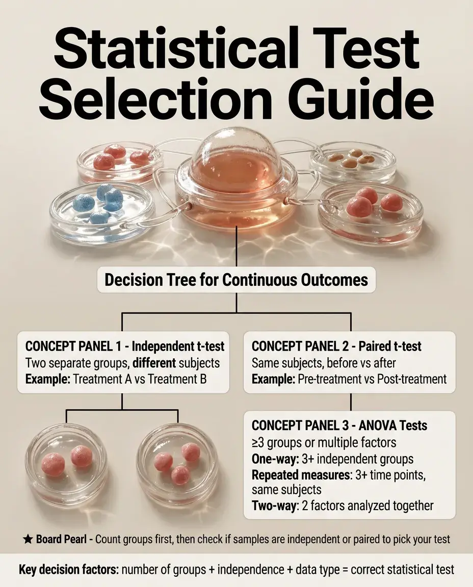
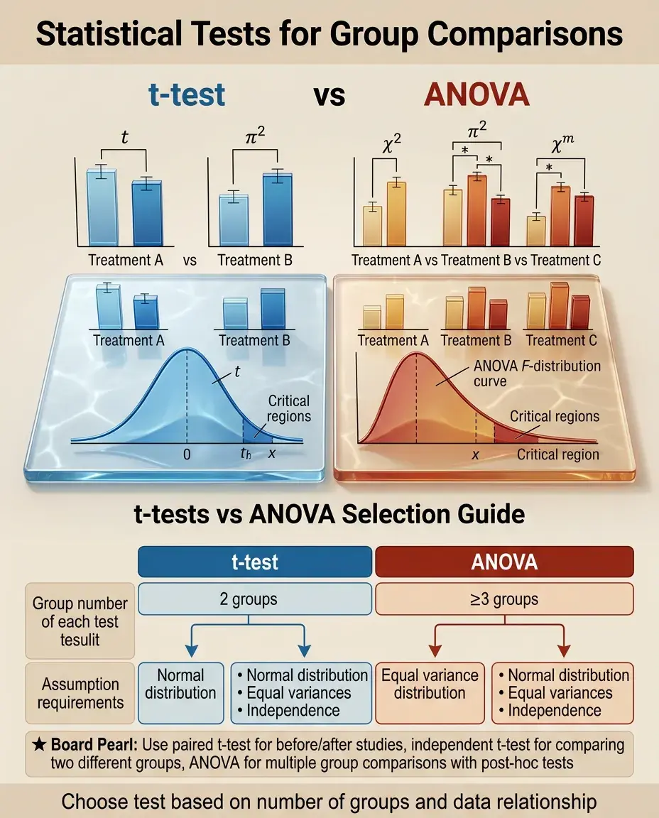
t-tests compare exactly 2 groups; ANOVA compares 3 or more groups simultaneously.
🧷
Board pearl: If comparing means of 2 groups → t-test. If comparing means of ≥3 groups → ANOVA.

The t-statistic: Signal-to-Noise Ratio
📍
t = (difference between group means) ÷ (standard error of the difference).
📍
Conceptually, t represents how many standard errors separate the two group means — larger t values indicate greater separation.
📍
The denominator incorporates both sample variability (pooled standard deviation) and sample size.
📍
Degrees of freedom (df) = n₁ + n₂ − 2 for independent samples, where n₁ and n₂ are the two sample sizes.
📍
Critical t-values depend on df and desired significance level (α, typically 0.05).
📍
Board pearl: Larger sample sizes → smaller standard error → larger t-statistic → more likely to detect true differences.

Independent (Unpaired) t-test
🔹
Compares means between two independent groups with no pairing or matching between observations.
🔹
Classic example: Comparing mean blood pressure between patients receiving drug A versus placebo, where different patients are in each group.
🔹
Assumes both groups are sampled from populations with equal variances (can be tested with Levene's test).
🔹
If variances are unequal, use Welch's t-test modification which adjusts the degrees of freedom.
🔹
Board distinction: Independent = different subjects in each group. No subject appears in both groups.

Paired (Dependent) t-test
⭐
Compares means between two related measurements on the same subjects or matched pairs.
⭐
Classic examples: Before-and-after treatment measurements on the same patients, left eye vs right eye measurements, twin studies.
⭐
Analyzes the mean of the differences between paired observations, not the difference between means.
⭐
More powerful than independent t-test because it controls for between-subject variability.
⭐
df = n − 1, where n is the number of pairs.
⭐
Board pearl: If the question mentions "same patients measured twice" or "matched pairs" → paired t-test.

One-Sample t-test
✅
Compares a sample mean to a known population mean or hypothesized value.
✅
Example: Testing if mean birth weight in a hospital (sample) differs from the national average of 3300g (population value).
✅
t = (sample mean − hypothesized mean) ÷ (standard error of the mean).
✅
Standard error = sample standard deviation ÷ √n.
✅
df = n − 1.
✅
Less commonly tested on boards but appears when comparing observed data to established norms or reference values.

ANOVA: Analysis of Variance Fundamentals
🧠
ANOVA tests the null hypothesis that all group means are equal: H₀: μ₁ = μ₂ = μ₃ = ... = μₖ.
🧠
Despite its name focusing on "variance," ANOVA is fundamentally about comparing means.
🧠
The test partitions total variability into between-group variability (signal) and within-group variability (noise).
🧠
F-statistic = (between-group variance) ÷ (within-group variance).
🧠
Large F values suggest group differences; F ≈ 1 suggests no difference.
🧠
Board pearl: ANOVA tells you if at least one group differs but doesn't identify which specific groups differ.

One-Way ANOVA
⚡
Compares means across ≥3 groups for a single independent variable (factor).
⚡
Example: Comparing mean cholesterol levels among patients on diet alone vs statin vs diet + statin (3 groups, 1 factor).
⚡
Between-group df = k − 1 (k = number of groups).
⚡
Within-group df = N − k (N = total sample size).
⚡
Results in an F-statistic with its associated p-value.
⚡
If significant, requires post-hoc testing to determine which specific group pairs differ.

Post-Hoc Testing After ANOVA
📌
A significant ANOVA indicates at least one group differs, but doesn't specify which groups.
📌
Post-hoc tests perform pairwise comparisons while controlling for multiple comparison inflation of Type I error.
📌
Common methods: Tukey's HSD (honestly significant difference), Bonferroni correction, Scheffé test.
📌
Bonferroni: divides α by the number of comparisons; most conservative.
📌
Tukey's HSD: balances Type I and II error; most commonly used.
📌
Board pearl: Without post-hoc correction, performing multiple t-tests inflates the chance of finding false positives.

Two-Way ANOVA
📣
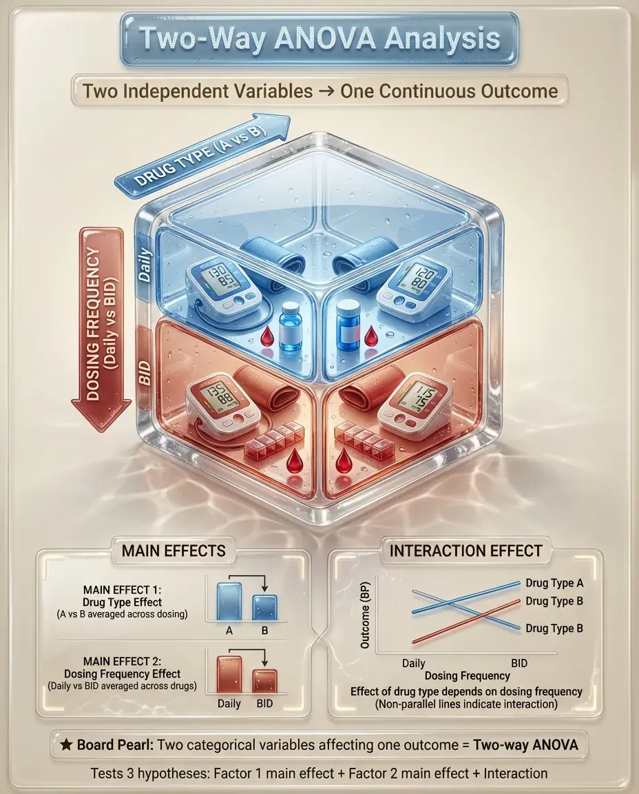
Analyzes the effect of two independent variables (factors) on a continuous outcome.
📣
Example: Examining how both drug type (A vs B) and dosing frequency (daily vs BID) affect blood pressure.
📣
Tests three hypotheses: main effect of factor 1, main effect of factor 2, and interaction between factors.
📣
Interaction means the effect of one factor depends on the level of the other factor.
📣
Board clue: If a question mentions examining two different categorical variables' effects on an outcome → two-way ANOVA.
Repeated Measures ANOVA
🔸
Extension of paired t-test to ≥3 time points or conditions on the same subjects.
🔸
Example: Measuring pain scores at baseline, 1 hour, 2 hours, and 4 hours after analgesia administration.
🔸
Accounts for correlation between repeated measurements on the same subject.
🔸
More powerful than independent groups ANOVA because it controls for between-subject variability.
🔸
Assumes sphericity (equal variances of differences between all pairs of conditions).
🔸
Board distinction: Same subjects measured multiple times → repeated measures ANOVA, not one-way ANOVA.

Assumptions and Violations
🧷
Normality: data within each group should be approximately normally distributed. Violated with skewed data or outliers.
🧷
Independence: observations must be independent. Violated with clustered data or repeated measures (unless using appropriate test).
🧷
Homogeneity of variance: equal variances across groups. Violated when one group has much more variability.
🧷
For t-tests, Central Limit Theorem helps with normality assumption if n ≥ 30 per group.
🧷
ANOVA is fairly robust to minor violations with equal sample sizes.
🧷
Board pearl: Severely skewed data or unequal variances → consider non-parametric alternatives.

Effect Size and Clinical Significance
📍
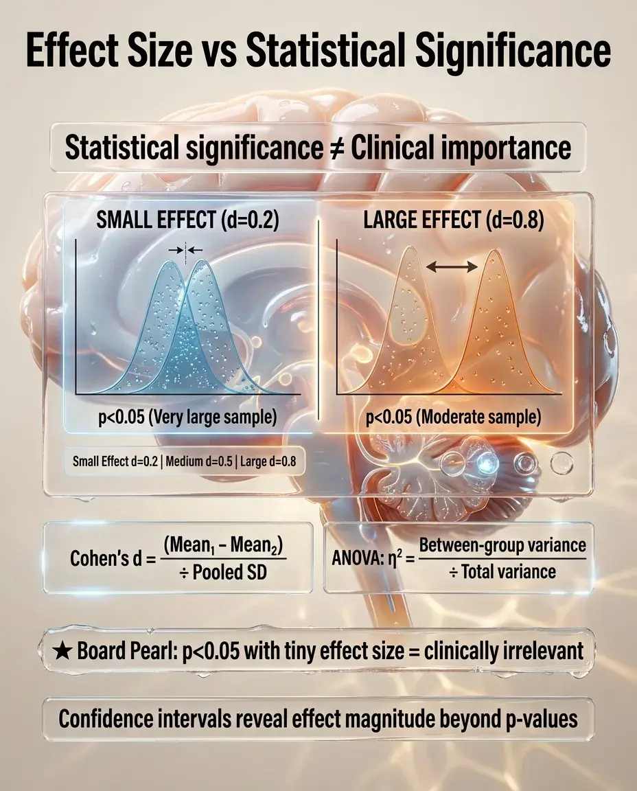
Statistical significance (p < 0.05) doesn't equal clinical importance — with large samples, tiny differences can be "significant."
📍
Cohen's d = (mean₁ − mean₂) ÷ pooled standard deviation.
📍
Small effect: d = 0.2; Medium: d = 0.5; Large: d = 0.8.
📍
For ANOVA, eta-squared (η²) = between-group variability ÷ total variability.
📍
Confidence intervals provide more information than p-values alone.
📍
Board principle: A statistically significant result with a trivial effect size may have no clinical relevance.
Sample Size and Power
🔹
Power = probability of detecting a true difference when it exists (1 − β, where β = Type II error rate).
🔹
Standard power target is 80%, meaning 20% chance of missing a true effect.
🔹
Factors increasing power: larger sample size, larger effect size, higher α level, lower variability, paired/repeated designs.
🔹
Sample size calculations require: expected effect size, desired power, significance level, and estimated variability.
🔹
Board pearl: Insufficient sample size → underpowered study → may fail to detect clinically important differences.

Type I and Type II Errors in Context
⭐
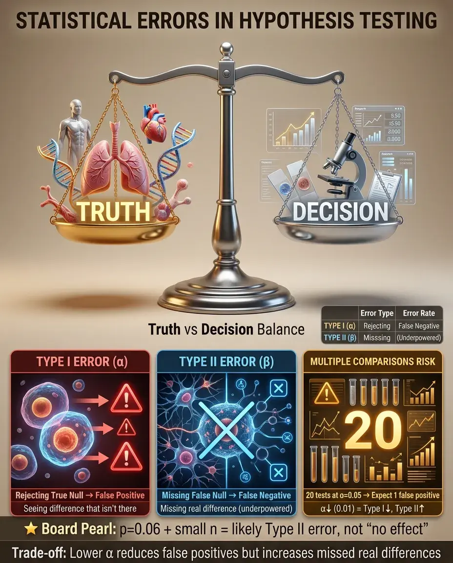
Type I error (α): rejecting a true null hypothesis — claiming a difference exists when it doesn't.
⭐
Type II error (β): failing to reject a false null hypothesis — missing a real difference.
⭐
Multiple comparisons increase Type I error risk: with 20 tests at α = 0.05, expect 1 false positive by chance.
⭐
Trade-off: lowering α (e.g., 0.01) reduces Type I error but increases Type II error.
⭐
Board scenario: A study with p = 0.06 and small sample size likely represents Type II error (underpowered), not proof of no effect.
Non-Parametric Alternatives
✅
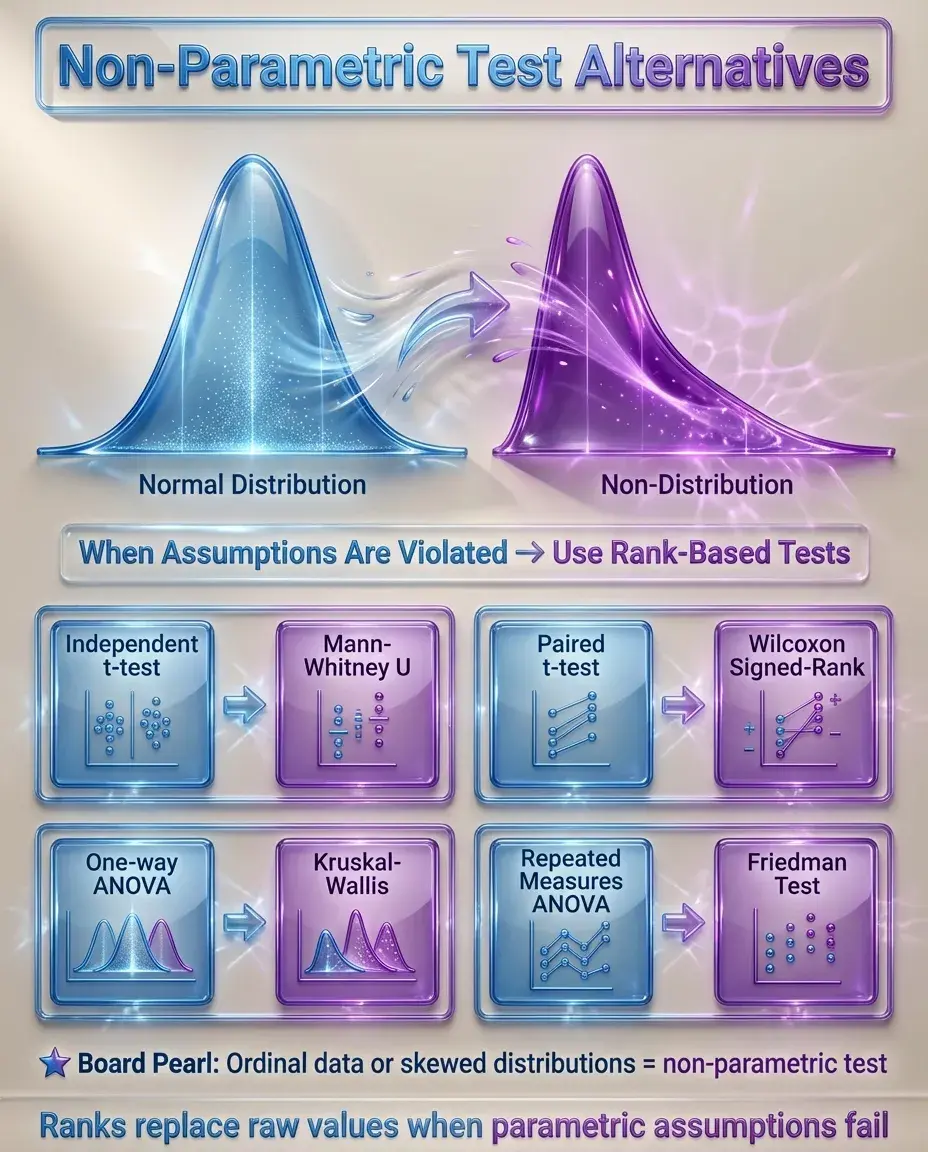
When parametric assumptions are violated, non-parametric tests analyze ranks rather than raw values.
✅
Mann-Whitney U test: non-parametric alternative to independent t-test.
✅
Wilcoxon signed-rank test: non-parametric alternative to paired t-test.
✅
Kruskal-Wallis test: non-parametric alternative to one-way ANOVA.
✅
Friedman test: non-parametric alternative to repeated measures ANOVA.
✅
Board pearl: Ordinal data (e.g., pain scales 1-10) or obviously skewed data → use non-parametric test.
Common Biostatistical Pitfalls
🧠
Multiple t-tests instead of ANOVA: inflates Type I error when comparing ≥3 groups.
🧠
Using independent t-test for paired data: ignores correlation, reduces power.
🧠
Ignoring assumptions: applying parametric tests to severely skewed or ordinal data.
🧠
Confusing statistical and clinical significance: tiny p-values don't guarantee meaningful effects.
🧠
Post-hoc data dredging: finding "significant" results by testing many hypotheses without correction.
🧠
Board warning: If comparing 4 groups with 6 separate t-tests → incorrect approach, use ANOVA.

Choosing the Correct Test
⚡
Two groups + continuous outcome + independent samples → independent t-test.
⚡
Two groups + continuous outcome + paired samples → paired t-test.
⚡
≥3 groups + continuous outcome + independent samples → one-way ANOVA.
⚡
≥3 time points + continuous outcome + same subjects → repeated measures ANOVA.
⚡
Two factors + continuous outcome → two-way ANOVA.
⚡
Violated assumptions or ordinal data → non-parametric alternative.
⚡
Board strategy: Identify number of groups, independence of observations, and data type to select the test.
Interpreting Results in Research Papers
📌
Check the p-value against the predetermined α level (usually 0.05).
📌
Look for confidence intervals — they provide both significance and effect magnitude.
📌
Verify appropriate test selection based on study design and data characteristics.
📌
Consider clinical relevance beyond statistical significance.
📌
Watch for multiple comparison corrections in studies with many outcomes.
📌
Board skill: Given a results table, identify whether the correct statistical test was used based on the study description.

Board Question Stem Patterns
📣
Comparing mean blood pressures between drug and placebo groups (different patients) → independent t-test.
📣
Comparing pre- and post-treatment weights in the same patients → paired t-test.
📣
Comparing mean healing times among 4 different wound dressings → one-way ANOVA.
📣
Study reports p = 0.15 with n = 10 per group → likely underpowered (Type II error).
📣
Comparing 5 groups with 10 separate t-tests → inappropriate, should use ANOVA with post-hoc tests.
📣
Severely right-skewed outcome data → non-parametric test needed.
📣
Both drug type and dosing schedule affecting outcome → two-way ANOVA.

One-Line Recap
🔸
t-tests compare means between 2 groups (independent for different subjects, paired for same subjects), while ANOVA extends this to ≥3 groups by partitioning variance into between-group and within-group components, with both requiring normal distributions and equal variances, using post-hoc corrections for multiple comparisons, and having non-parametric alternatives when assumptions are violated.
bottom of page